Visualizing Patient Origin in North Carolina Using Zipcode in R

Tianyi Liu

October 02, 2023 September 23, 2024

Do you want to plot something like this? Wonder how you could do it in R?

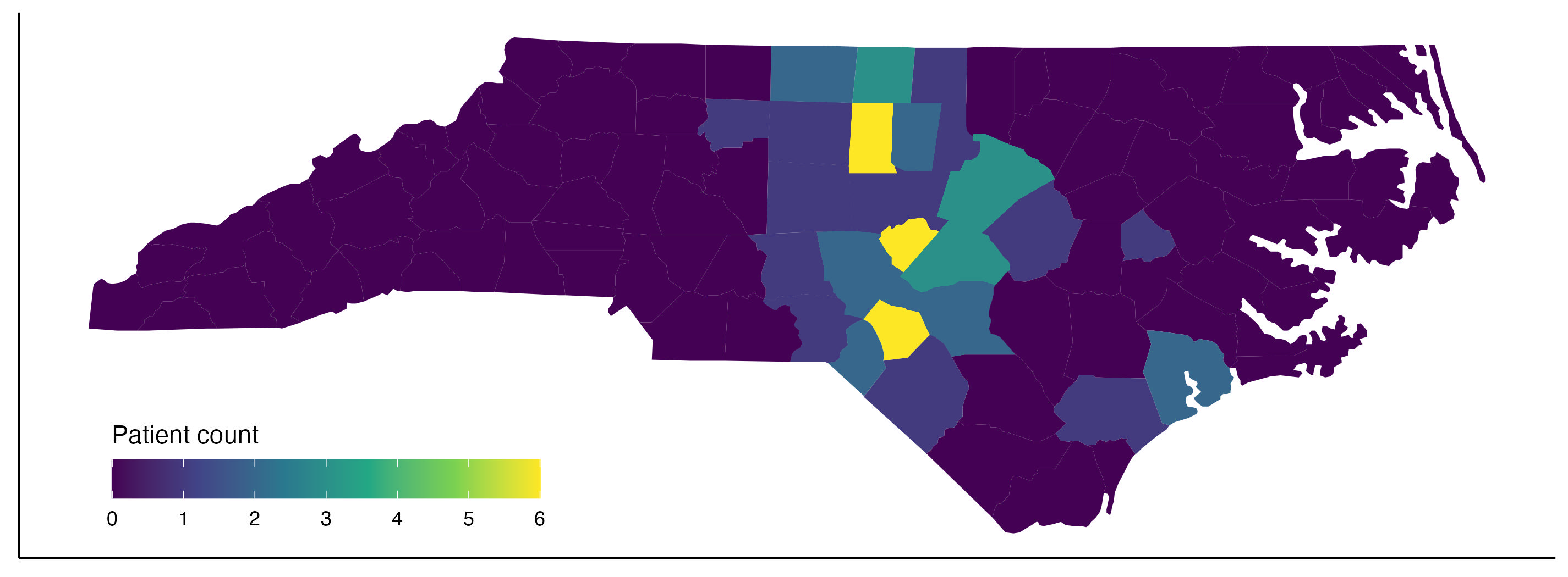
In this article, we will go over in detail the steps for plotting the density of patients from each North Carolina (NC) county by their zipcode using ggplot in R, a.k.a. the plot above. We have 191 patients from 57 unique zipcodes. Since the patient data are protected, the full data is not presented here. You can find the zipcode data by clicking here.

The main workflow here it to merge the data frame containing patient count by county with that of the map coordinates of each NC county. Some data wrangling is needed to translate patient zipcode to county names before the final merging of the data frames. Some contents of this blog post are inspired by this post by Peter Haschke.

This post assumes that you have a beginner knowledge of R and its data wrangling functions in tidyverse, as well as the pipe operator. If not, these links will provide you with some refreshers!

We start by loading the following packages in R:

library(dplyr) # data wrangling
library(stringr) # string object manipulation
library(magrittr) # the package of the famed pipe operator
library(ggplot2) # data plotting
library(grid)
library(maps) # this allows us to extract NC map
library(scales)
library(zipcodeR) # for zipcode metadata
library(ggthemes) # not necessary - allows us to set ggplot themes more easily

Suppose that the patient data is stored in a tibble named clean_df, where there is a column zip that contains all the zipcodes:

head(clean_df %>% dplyr::select(zip), 5)

# A tibble: 5 × 1
   zip  
   <fct>
 1 28376
 2 28376
 3 27278
 4 28315
 5 27616

Now, we count up the number of patients from each zipcode using the summarise() function:

zip_sum <- clean_df %>%
  group_by(zip) %>%
  summarise(n = n()) %>%
  ungroup
head(zip_sum, 5)

# A tibble: 5 × 2
   zip       n
   <fct> <int>
 1 24112     1
 2 27025     2
 3 27105     1
 4 27208     1
 5 27215     8

After this, we can map the patient zipcodes to their metadata

zip_info <- reverse_zipcode(zip_sum$zip)

A sample of this zip_info data frame should look like this (by calling head(zip_info, 2)):

# A tibble: 2 × 24
  zipcode zipcode_type major_city    post_office_city  common_city_list county  state   lat   lng
  <chr>   <chr>        <chr>         <chr>                       <blob> <chr>   <chr> <dbl> <dbl>
1 27025   Standard     Madison       Madison, NC             <raw 19 B> Rockin… NC     36.4 -80  
2 27105   Standard     Winston Salem Winston Salem, NC       <raw 25 B> Forsyt… NC     36.2 -80.2

The only conlumns we want are zipcode and county. We also rename zipcode to zip to be consistent with the variable name in zip_sum:

zip_sub <- zip_info %>%
  dplyr::select(zipcode, county) %>%
  rename(zip = zipcode)

Next, we begin by extracting the NC county map coordinates from the map package, and save it in a data frame for plotting later:

map <- map_data("county")
nc <- subset(map, region == "north carolina") # subset the data to NC county coordinates

We can check the head of nc as well (head(nc, 2)):

long      lat group order         region subregion
54915 -79.53800 35.84424  1857 54915 north carolina  alamance
54916 -79.54372 35.89008  1857 54916 north carolina  alamance

A little bit of geographical knowledge tells us the county names are stored in the column named subregion, and they are all lower-case while without the trailing “County” as in zip_sub! To match this, we make some changes to the column storing county names in zip_sub:

zip_sub <- zip_sub %>%
  # extract county names and set the first latter to lower case
  # assign these values to the column 'subregion'
  mutate(subregion = str_split_i(county, " ", 1),
         subregion = str_to_lower(subregion)) %>%
  dplyr::select(-county)

Now, we are ready to merge zip_sub with zip_sum, which yield each patient’s county of origin; and then we merge this combined data frame with nc, adding the map coordinates for counties:

pt_zip_counts <- zip_sum %>%
  left_join(zip_sub, by = "zip") %>%
  right_join(nc, by = "subregion", relationship = "many-to-many")

This prompts many missing values NA since we do not have any patient from the majority of counties. To deal with this, we just replace the missing value with 0:

pt_zip_counts$n <- replace_na(pt_zip_counts$n, 0)

The following steps are also not mandatory: we replace any count of patients from a zipcode above the 95-th percentile of all counts to the 95-th percentile value to get a better dynamic range of colors - this way low counts like 1 would be clearly visualized as well.

pt_zip_counts$n_plot <- pt_zip_counts$n
pt_zip_counts$n_plot[pt_zip_counts$n_plot > quantile(pt_zip_counts$n, .95)] <- quantile(pt_zip_counts$n, .95)

A final check of the data frame (head(pt_zip_count, 2)) shows the followings:

# A tibble: 2 × 9
  zip       n subregion   long   lat group order region         n_plot
  <chr> <int> <chr>      <dbl> <dbl> <dbl> <int> <chr>           <dbl>
1 27025     2 rockingham -80.0  36.5  1937 57960 north carolina      2
2 27025     2 rockingham -79.7  36.5  1937 57961 north carolina      2

Now, we dish up the plot using geom_polygon from ggplot:

S <- ggplot(data = pt_zip_counts) +
  geom_polygon(aes(x = long, y = lat, group = group, fill = n_plot)) +
  scale_fill_viridis_c("Patient count") +
  theme(axis.text = element_blank(),
        axis.ticks = element_blank(),
        axis.title = element_blank(),
        panel.grid = element_blank(),
        legend.position=c(.2,.15)) +
  guides(fill = guide_colorbar(barwidth = 13, title.position = "top", direction = "horizontal"))

Saving it using the following line (you can substitute the file path with whatever you like):

ggsave("patient_origin_map.png", S, width = 9.5, height = 3.5)

We have the final product shown at the beginning of the page!

Thanks for reading! I hope you have learned a lot and enjoyed this content. Have questions or suggestions? Feel free to email me through the Contact page.